Jianhong Wu, Zachary McCarthy, Michael Glazer
Background
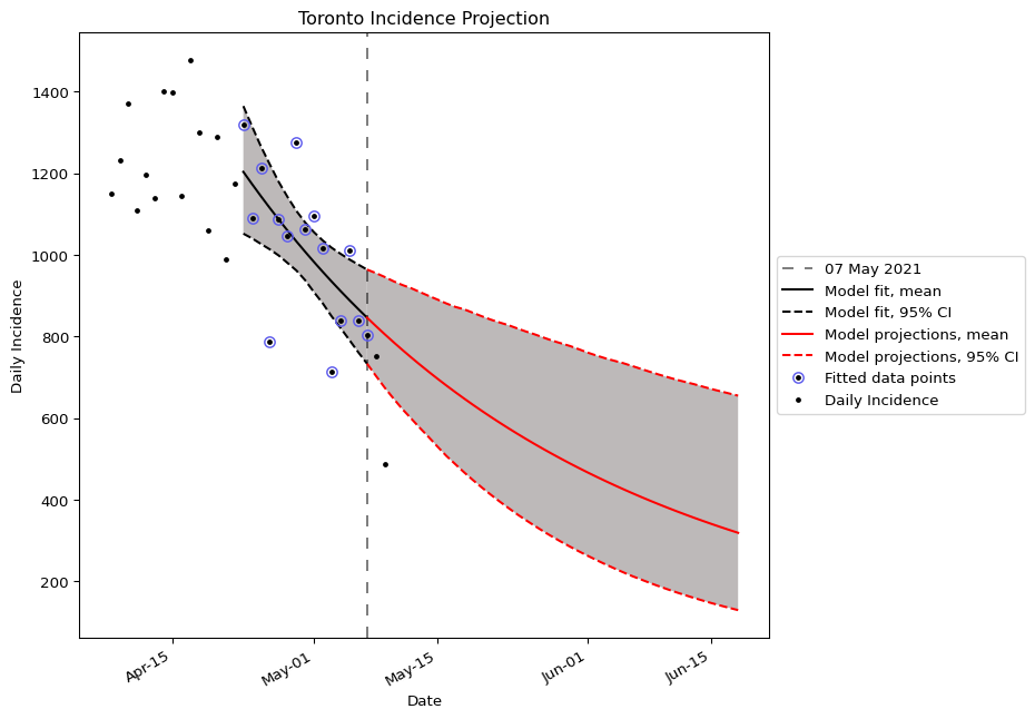
This report presents a forecast of the number of COVID-19 cases reported in the Toronto public health unit (PHU) in Ontario, Canada. The fitting results and forward projection are provided, as well as the parameter estimates for the mathematical model underlying the projections. An outline of the assumptions and methodology used to produce the forecast are included below.

Assumptions
The main modelling assumption is that the number of newly reported cases each day is generated by an exponentially growing mean. This is combined with the negative binomial probability distribution function to construct the likelihood function over the observations during the fitting window.
Note: the projection reflects the scenario where the current interventions remain in place.
Methods
We fitted the exponential growth model y(t) = y_{0}e^{rt} to the daily reported cases in Toronto. We fitted the daily reported cases from 23 April, 2021 to 7 May, 2021 (n = 14 data points), or 2 weeks, to estimate the model parameters. For the parameter estimation, we used the maximum likelihood method with negative binomial likelihood. The method is as follows:
First, the negative binomial probability distribution function (pdf) is given by
NB(k|n, p) = \binom{k + n - 1}{n - 1} p^{n} (1 - p)^{k}.We, instead, utilized the parameterization of the negative binomial distribution in terms of its mean μ and variance \theta \mu, i.e.,
p(\theta) = \frac{1}{\theta}, n(\mu, \theta) = \frac{\mu}{\theta - 1}.The mean value of y_{0} was assumed to be growing exponentially, that is, \mathbb{E}(y(t)) = y_{0}e^{rt}. With these assertions in place, the likelihood function over an observation period of n days is then
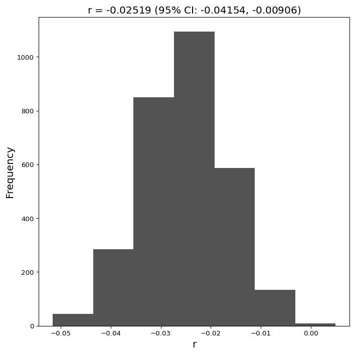
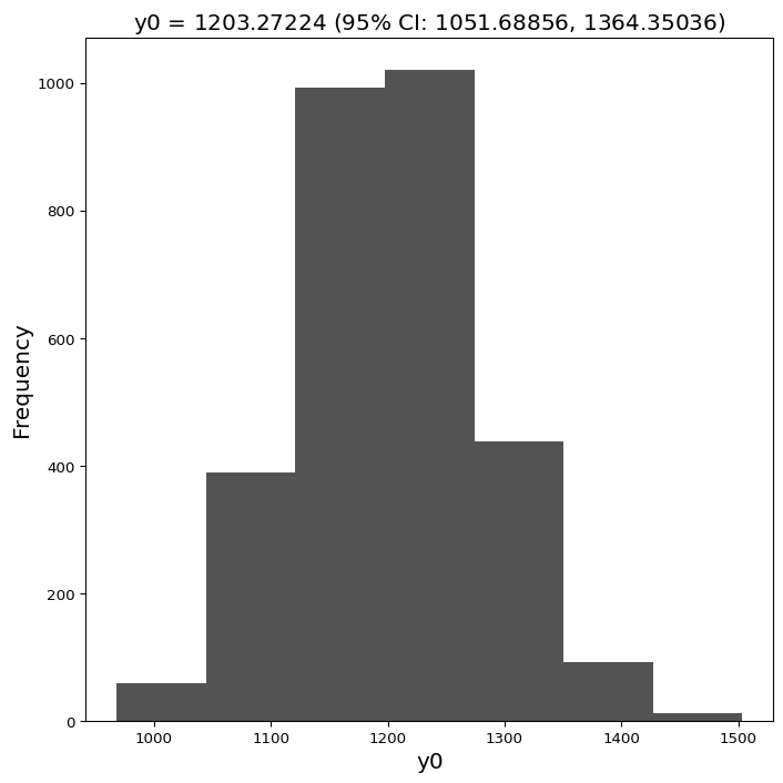
L(y |y_{0}, r, \theta) = \prod^{n}_{i}NB(y(t)|n(y_{0}e^{rt}, \theta), p(\theta)) = \prod^{n}_{i}NB(y(t), \frac{y_{0}e^{rt}}{\theta - 1}, \frac{1}{\theta}).We maximized the negative log likelihood using the Python package scipy's functions fmin and gammaln (to emulate the optimization procedure fmincon in Matlab) to estimate the parameters y_{0}, r, \theta. Note that in addition to the parameters associated with the exponential model y_{0} and exponential growth rate r, the dispersion parameter associated with the negative binomial distribution \theta was also estimated.
Using the parameters obtained y_{0}, r, \theta, we constructed N = 3000 re-sampled time series all of identical length n = 14. For each re-sampling, we performed the parameter estimation process specified above to obtain a corresponding estimate of y_{0}, r, \theta. We therefore obtained a set of parameter N estimates, which gave an empirical distribution of the parameters and a corresponding set of N exponential projections for the future.
The final projection for Toronto was obtained by taking, for each day in the future, the mean of the set of projections obtained through bootstrapping, and 95% confidence interval obtained by taking the 0.025 and 0.975 quantiles of the same distribution.
Data
To parameterize the model, we utilized the list of confirmed positive cases of COVID-19 in Ontario according to public health unit. The time series of the daily cases of COVID-19 in Toronto was generated using this individual line listed data from the Ontario Ministry of Health, which was made available to us through the Ontario COVID-19 Modeling Consensus Table. This main source of data enabled the fitting of mathematical model and the subsequent projections.